Well, I had a really great text for this, but it got deleted on the writing process. Already 900 words going, that will never come back. It left me frustrated, but well, I guess I just have to do it again. Prepare this month for something that brings together some stuff you learned in high school and will, hopefully, change the way you see yourself.

So, today we will begin with a different topic, enough rambling about general physics, let’s look at some other sides. I like space but I am not an astrophysicist, I like particle physics, but I don’t see myself working there. I need to work on something that clicks with me. Speaking about clicking, isn’t it funny whenever someone has an idea, old cartoons showed a light bulb. It really makes you wonder, what would they be drawing before lightbulbs, candles? If you were to look at your brain, you could see (well, not actually see, but measure) tiny potentials going all the way, like tiny light bulbs.

Hey, that gave me an idea, let’s talk about brains. My professor likes to say that brains are “The most interesting and complex kilogramme of matter in the universe“. And it really makes you wonder what makes brains so fascinating in the first place? It is certainly not any new physics, the particles and fundamental interactions, are the same ones, that everyone is used too, and if you are a particle physicist, brains are the most boring things you can imagine. But I’m not a particle physicist, so I don’t care about that. A lot of the most interesting things in nature require relatively simple physics (but not simple mathematics, may I add), and by simple physics, I mean, you don’t have to consider quantum effects nor relativity (both kinds). So what makes the brain so interesting? A lot of things, but that would be too long to cover in a single post, and from the analytics I can see that long posts are not the best, even for an entire month. So let’s do like neuroscientists, and start from the bottom by talking about the single neuron. (PS: Hope you have your biology classes from high school in check, because that’s all you need).

So, a neuron has all these parts, but really, you only need to focus on these:

• Cell  body (or soma in some books)
• Nucleus
• Dendrites (Receives info from other neurons)
• Axons (Sends info to other neurons, may or may not be covered in myelin sheaths).

And sure many of those structures are important, but since we are only talking about a single neuron right now , it is not really necessary for us to think about dendrites and axons. Just imagine a cell for now, and let’s zoom a little bit further, so we can now see those big macromolecules like proteins and stuff. And let’s look at what keeps the inside of cell isolated from the outside.

Again, a quick youtube video might help you recall this, but there we go, a membrane.

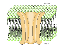
A cell membrane is made of a lipidic bi-layer that is hydrophillic (likes water) in the middle and hydrophobic (doesn’t like water) on the outside. Sometimes it has some proteins crossing it, and those proteins may serve as channels that allow some molecules (or ions) to pass. Others may also be receptors and pumps. But today we’ll focus mostly on the channels, specifically the ion channels in neurons for sodium and potassium.

But first let’s talk about particle flow. Let’s say you had a container divided in two sides by a thin, impermeable membrane , one side has water with red corant, and the other has water with some blue corant in it.

What you happen if you were to put a small hole in the membrane? It is not crazy to say, without any other prior info, that at the end of a certain time, both side of the container would have the same colour, and that colour would be pink (or purple, depending on the ratio of red to blue). And that is pretty intuitive. And after that happens, it’s also safe to say that after a while the colour for each side won’t go back to being red and blue. So it’s like the state where both sides are coloured pink, would be at a sort of equilibrium.  You can think of red and blue corants as being a bunch of red and blue particles, and essentially the equilibrium state is when the concentration of red and blue particles on both sides are equal. But how does it happen, and why is that? These questions are relevant for physicists. And questions like these were part of the revolution in the late 19th and early 20th century. And as with many questions in statistical mechanics, it somehow comes back to entropy.

Now, entropy is kind of a funny concept. We learn it to be the measure of “disorder” of a system. Although that is not really accurate.  Entropy is defined more has a representation of the microstates of a system. And what are microstates? They are what we can call all the different configurations of a system.

The best example we can think of it, is for you to imagine a chess-board. And imagine that chess board to have only a single square. You have a pawn. In how many squares can you have the pawn? In this case, only 1.  But if you increase the number of squares, to let’s say, 4, now your pawn has more possible squares to be in, and has such, your system made by the board and the pawn, have more configurations or microstates, and higher entropy as a result. Realize that neither system is more or less organized then the other. So, when the second law of thermodynamics says that the entropy of a closed system increases, well, that just means that the number of configurations of all the particles that make up that system increase over time, and it either increases or remains constant. The entropy is just a quick way to know the configuration of a system. And it is more useful to look at change in entropy than to look at entropy itself. And it is that change in entropy that is represented in the second law, explicitly as

See, very easy. As to why things tend to spread out like that, “diffusing” in some medium, it is because of this change in entropy. Or better, this change in entropy reflects what is going on the system. On our earlier example, before having a hole on the membrane, the two systems were isolated, and all possible configurations were being displayed for that cases, but after the hole, now you have a whole new space that didn’t have any red/blue particles, and now you have new possible configurations to explore, and so the particles spread out, and by spreading out, they increase the entropy of the system. By the way, the expression for entropy (in the context of statistical physics) is:

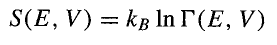
That weird symbol there is the volume of the microcanonical ensemble which is the ensemble for all configuration for an isolated system. Why are we using a logarithm of that? For a typical system of particles you may have 10 to the power of 23 particles (or 1 with 23 zeros behind it), and that implies a huge number of possible configurations. Let’s use 4-square chess-board and two pawns (one black and one white):

• You have 4 states for each piece, where the board only has one pawn;
• You have 12 possible states when the board has  two pawns;
• You have one state where the board is empty;

With just two pawns, and a 4-squared board, the total system has seventeen possible states. Imagine with 1 sextillion particles. It is better to use logarithms to show the values in a number that is more understandable. And the constant in front is the Boltzmann constant, it shows up all the time in thermodynamics, and statistical physics.

And that explains why, but it doesn’t really explain how. To describe that we need to understand “diffusion”. The first question that pops out is, “What is diffusion?”. Well, diffusion is really just the process of moving from a point of higher concentration to one of lower concentration, a process that would only stop if everywhere where it happens were to be in equilibrium. That is a rather limiting definition, because we still are left with questions as “Why does it have to be from somewhere with higher concentration to somewhere with lower concentration?” . So a couple of people worked on finding a better definition, for this diffusion, that is so ubiquitous to all processes in nature. And this is where they came up with the concept of brownian motion.

Fun fact: Brownian motion was first observed in detail by Robert Brown, a botanist, while observing a small polen grain through a microscope. He noticed that the polen was moving around in a random manner, and initially he thought it was due to some living process, however after careful experiments, he determined the process to be purely physical.

This brownian motion is the random motion of particles (be it small grains, sand, or even smaller, like molecules or ions) through a certain medium. For a long time after Brown published it’s results it was unknown why such a random motion would occur. Many theories were postulated, and back people were still debating the existence of atoms, some physicists thinking of them just as quirky mathematical tricks, while others would be thinking of them as being tangibly real. In 1905, in one of his annus mirabillis papers, Einstein published about the Brownian motion, describing the motion by the polen has been due to the collision it suffered with the water molecules (a single water molecule may not be able to push you around, but a bunch of them? Maybe!–), further cementing the discussion in favour of the atomists. Perrin verified it experimentally (and he won a Nobel for it).  The multiple collisions between multiple particles would make them move randomly and turns out their motion is not fundamentally random, but the shear number of molecules is definitely more than any computer can be able to predict. So, yeah, you can’t really predict how a single particle might move. But you can calculate the probability for it to be at a certain location at a certain point in time.

And that probability follows a very well known distribution, so known and so common, people call it “normal” distribution – or Gaussian distribution, something like the following expression:

The expression itself is not what you need to know. What is the takeaway message you need is that this says that things tend to spread over a certain space, and that we know how it spreads over time.

That D is the diffusivity constant, and it typically depends on the materials. It determines how much something would spread or diffuse over some material. For example, a smaller D means that it will take longer for something to spread over some other thing, a bigger D means it will take a shorter time.

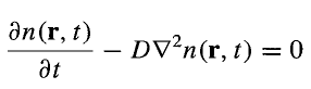
The truth is, that is just for the simple case where at time 0 everything is concentrated at a single point, so in reality, things are not as straight-forward. So what can describe a random motion? Really anything that satisfies the diffusion equation:

First consider Fick’s law:

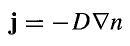
What this expression is telling you is that the current (the number of particles crossing some area over a certain period of time) of particles is directly proportional to the change in density of particles in each point in space (that is the bigger is the difference in density between two points in space, the higher is the current, or you have more particles going there). The proportionality constant is our old friend D, and the minus sign means it goes towards the place with lower density. This law is the mathematical shorthand for everything we said before, about how particles tend to flow from a place with high concentration to a place with lower density.

The diffusion law is just a continuity equation, saying “Hey, I get it that you need to go somewhere, but it’s not we have an infinite number of particles, you know? Like, you need to know that at one point you won’t have anything else to send” or something like that.

It can be written like:

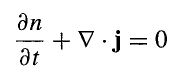
Again, this means as you have a current (if you want to know a bit more about currents, check my post on Noether’s Theorem) taking things from point A to point B, things in point A will change over time, just like the current will change between point A and point B. But since you need to remain with the same number of particles (if you are in an isolated system), if you combine all the changes in your system, it should add up to zero. It’s the good ol’ conservation of mass.

And since we don’t really like dealing with two unknowns (n and j) we need to get rid of one of them. Now you use Fick’s and voila, you get a pretty reasonable and short formula:

And with this expression, you can find any possible distribution for your Brownian motion, and your diffusion pattern. By the way, the diffusivity constant can be determined by the Einstein Relation:

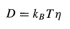
With this relation, you can find a bunch of variables that can influence how diffusivity is affected. T stands for temperature (in Kelvin) and essentially, it implies that higher temperatures increase diffusion (which is kinda intuitive when you think about it). That weird symbol, η, is the mobility of the particle, and it depends on many factors (and even what kind of particle is being diffused).

Note: In reality the diffusion is a constant only in very particular cases, and in more general cases, it’s a second-rank tensor. 

Now, with this, you essentially know how particles flow from one place to the other, and how flow occurs across membranes. But, I need to come up clean with you guys about something. These equations, while being good and all for describing diffusion, are not enough to describe what happens at the membranes of our neurons. Don’t get me wrong, this describes the movement of particles and many other things, but to describe the action potential in neurons, we need to know the movement of ions, and ions have electric charge, which introduce an extra thing we didn’t consider before.

First, we were considering the flow of particles as being purely motivated by concentration gradients, moving from more to less concentrated areas. But for ions, that is only one of the acting “forces”. Having electric charges, that means they are susceptible to electrostatic forces and electric potentials, which do exist in cells. That has a big impact in their movement. The good thing is that not a lot of things need to be changed. (This is what happens if you don’t plan things ahead, you end up writing a huge text, only to debunk yourself by the end). First, let’s go the place where we had Fick’s Law. There we said the current only depended on the number density gradient, but we now agree that is not exactly the case for ions on a neuron membrane. Actually the expression was incomplete from the start. Let me number the two things we didn’t consider. First, we didn’t consider the motion of the fluid itself, and assumed that only the particles were flowing. Second, we didn’t consider the electric potential that could exist between two points. If we were to consider both cases, Fick’s Law would become:

The u term is the velocity of the fluid in which the particle is diffusing (if it is not a fluid, it becomes zero). And the extra term takes into account the electric force, that is defined by the charge of the ions (z times e, which is the elementary charge), times the electric field E.

Which would reflect itself in the expression for the diffusion equation as:

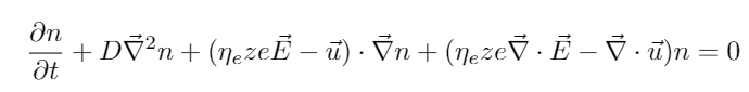
Pretty nasty, right? This doesn’t look appealing at all. But, there are some simplifications we can make, just by assuming that actually in the context of cell membranes, the fluid doesn’t move (what is physics we call stationary), meaning that u is equal to zero.

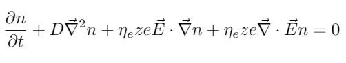
Still not that attractive, I’ll admit, but now, you only have to solve for n and E, and you don’t have to consider all the mess that comes from fluid mechanics (believe me, it is a huge mess). But still you may be rightful to think this isn’t pratical. And besides we didn’t even express the electric field in terms of its potentials (because that would also make a mess). This is known as the Nernst-Planck Equation, and this is a particular form of a much more complicated differential equation, a stochastic differential equation know as Fokker-Planck Equation (yeah, that Planck, and he will show up again in this post).

After all this rambling, maybe it is worthed to go back to our modified Fick’s law.  Some things for us to consider:

• The fluid is stationary (u is equal to zero), because of our prior conditions
• The electric mobility is described by the Einstein Relation.
• Let’s assume an electrostatic approximation (since the potential difference is generated by the different concentrations of ions on each side of our membrane), so that our Electric field is only dependent on a scalar potential, ultimately leaving us with:

And while you may think, “Uh, how does this help me in any way?”, there are many things you can do just with this expression. For instance, we may want to know what happens in the stationary flux (where j is equal to zero), or where the system is at an equilibrium – Nernst Equilibrium. It is important for us to know the properties of the system at equilibrium because that’s how the neuron typically is when it is not firing action potentials. While that may seem like a hard problem we can find an actual solution for our electric potential. With a couple of algebraic manipulation (also we replace D with the equivalent expression given by the Einstein Relation) we find:

Now this is amazing, because it gives us a way to describe the flow of particles across the membrane by just knowing the potential between the two sides. And it shows that for the equilibrium you may not have the same concentration of particles on both sides. Just by introducing an extra factor our equilibrium changes. And this expression depends on temperature, which is closer to your familiar expressions in thermodynamics. And we got here by using tools developed in other sides of physics, showing how intersectionality is important in this field. On a future post, we’ll use the conclusions from this post to derive the rules behind the propagation of information in our nervous system.

References:

• Kandel, Eric R., et al., eds. Principles of neural science. Vol. 4. New York: McGraw-hill, 2000.
• Nelson, Philip Charles, et al. Biological physics: energy, information, life. No. QH505 N44. New York: WH Freeman, 2008.
• Malmivuo, Jaakko, and Robert Plonsey. Bioelectromagnetism: principles and applications of bioelectric and biomagnetic fields. Oxford University Press, USA, 1995.